Ron Goetz and I have developed a technique and Mathematica package (called ContoursAndFlows) to show the surface that is the graph of z = f(x, y) by setting up a coordinate system based on contours and the curves orthogonal to them (flows: the paths a drop of water would take under gravity). This allows us to get very good images of graphs that are difficult, or impossible, to see using standard Cartesian grids. (References: Our two articles in Mathematica in Education and Research) Here are several examples.

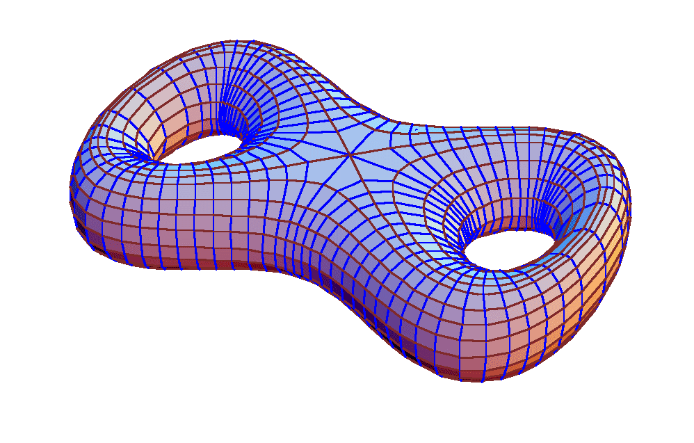
A Double Torus

A double torus can be obtained by plotting the following function (thanks to H. Karcher):

     z = Sqrt[-x^4 + 2*x^6 - x^8 + 2*x^2*y^2 - 2*x^4*y^2 - y^4 + (2/10)^2]

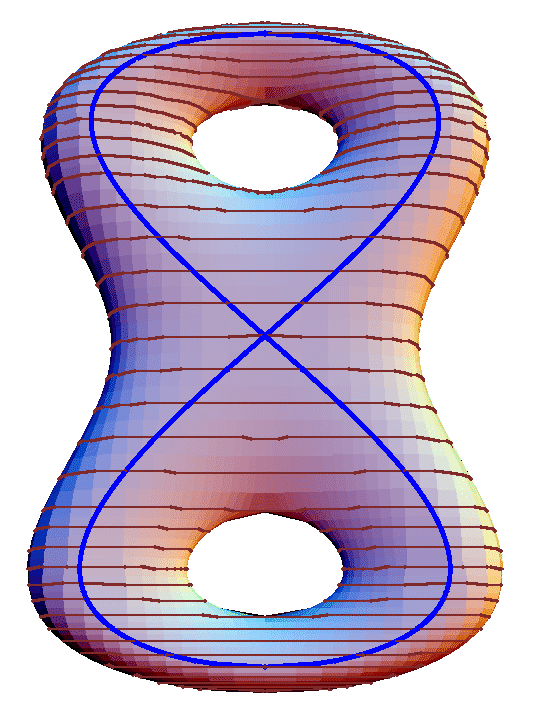
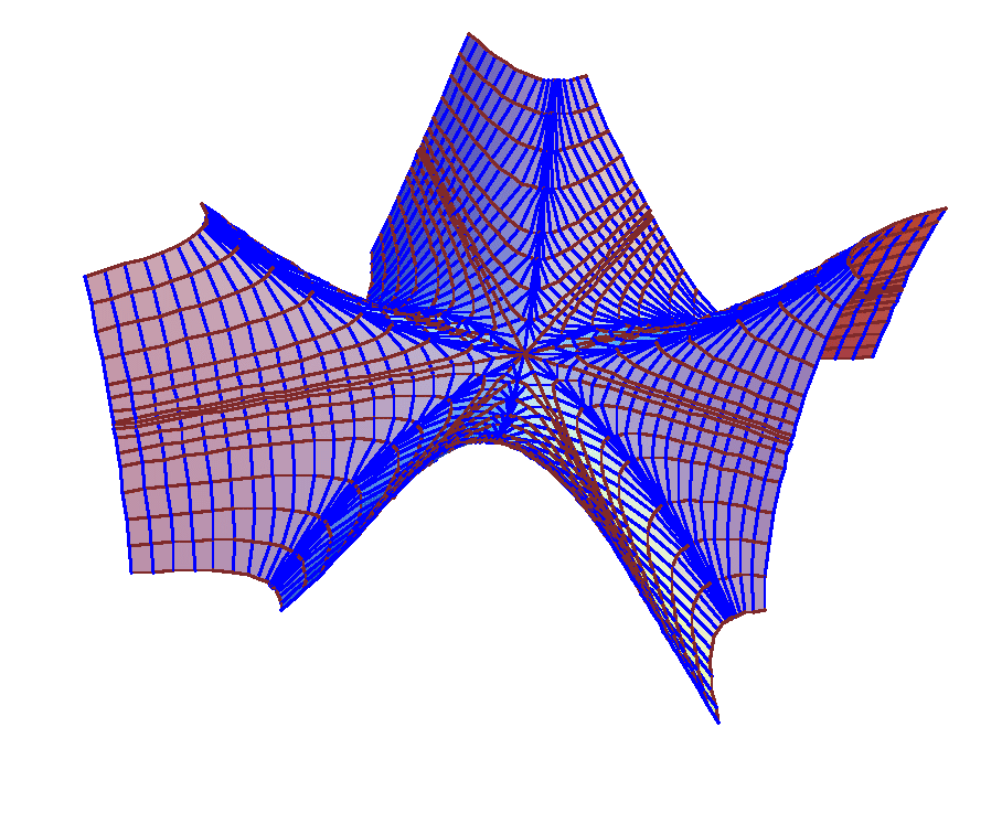
A Double Torus, Oriented Vertically

This image is shown with the contour lines only; some manual adjustments caused distortion in the flow lines, so I suppressed them. In any case, I think the contours are of more interest here. The figure-8 is added just no disguise the joins. This surface is obtained by pasting together -- very carefully -- the graphs of the eight functions:    w Sqrt[1/2 + w  Sqrt[5 - 20*y^2 + w 4*Sqrt[1 - 25*z^2]]/(2*Sqrt[5])], where the w's can be, independently, +1 or -1 (hence 8 choices). Each graph was obtained by the contour-and-flow method, but the flows were erased.

A Fubini Example

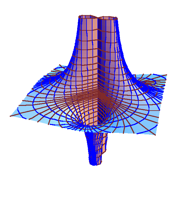
z = (x^2 - y^2) / (x^2 + y^2)^2 (from a paper in College Math. Journal (1998) by Hern, Long, and Long, who used it as an example related to Fubini's Theorem). In a rectangular plot the pieces do not touch properly at the z-axis.

A Flattened Sphere

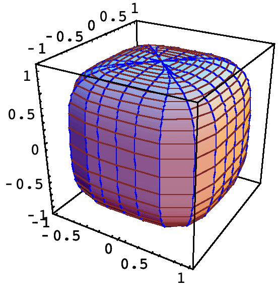
z = (1-x^4-y^4)^(1/4). Euler conjectured that, except for trivial cases, no three fourth powers could sum to a fourth power. He was wrong. Thus there is a nontrivial rational point on this surface.

Straight and Parabolic Limits

Here z = x^2 y / (x^4 + y^2), the classic example of a discontinuous function whose straight-line limits into the origin are all 0, but which has different limiting values on each parabola. The parabolic contours are evident in the image. We first generated the graph using closed forms for the parabolas and ellipses that form the contours and flows, but it is more general to use numerical methods, and that is how the present image here was done. The contours are color-coded from cyan to red to aid the visualization of height. As with many of our examples, a plot using standard rectangular coordinates is totally unsatisfactory.

Unequal Mixed Partial Derivatives

The classic example: z = x y (x^2 - y^2) / (x^2 + y^2), with different mixed partial derivatives at the origin.

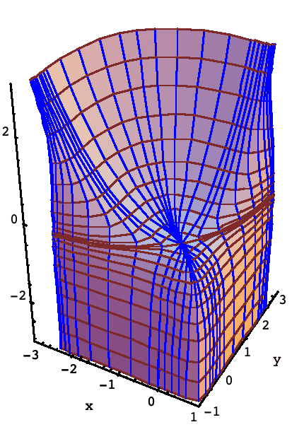
Discontinuous, But Partial Derivatives Exist

z = (1/4) [1 + (x^2 + y^2)^(3/2)] cos(4 arctan(y, x)), from Calvis, College Math. Journal, Jan 2000. It is discontinuous at the origin but has partial derivatives everywhere.

Failure of the Only-Critical-Point-in-Town Test

Here is  a polynomial example of the failure of the only-critical-point-in-town test. There is a local minimum, it is the only critical point, but it is not an absolute minimum. This function, found by Calvert and Vamanamurthy, is simply z = x^2 (1 + y)^3 + 7 y^2.

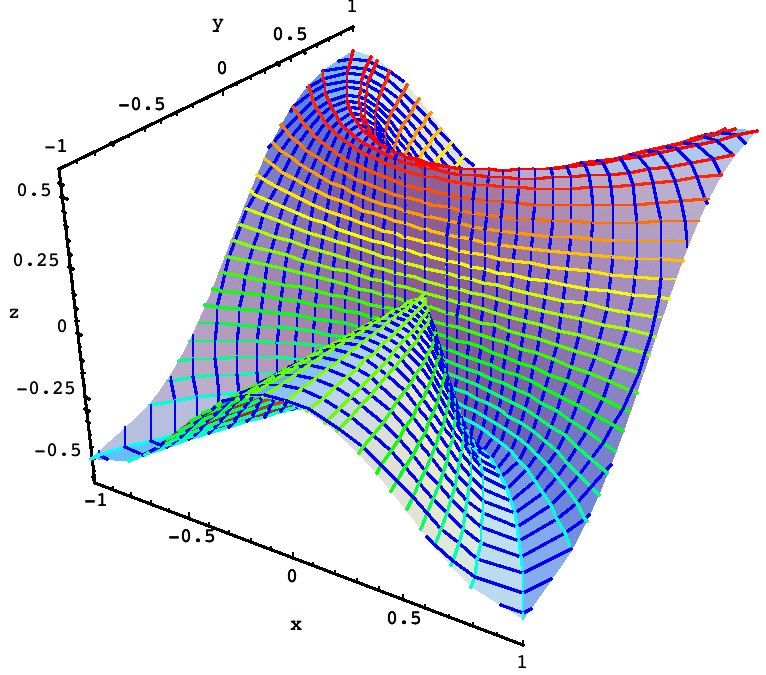
An Illustrative Example

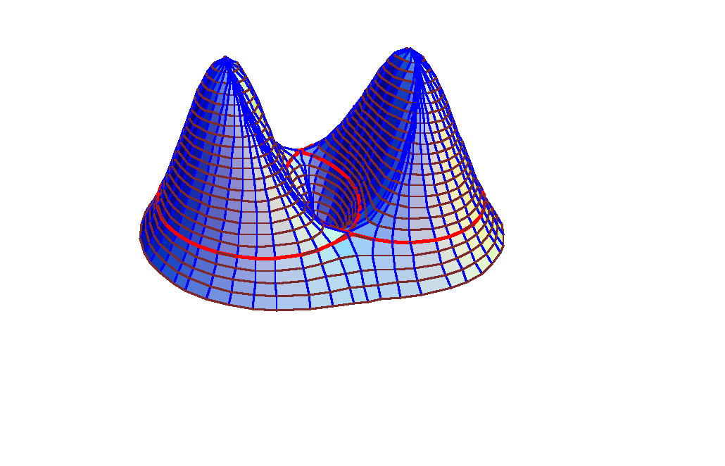
This is a function with two maxima, a minimum, and two saddles, and illustrates that the method can paste everything together nicely. The z = 1 contour is enhanced. The function is (x^2 + 3 y^2) e^(1 - x^2 - y^2). Note that the footprint coincides with a contour, which is typical of our method and is better than the usual rectangular footprint.

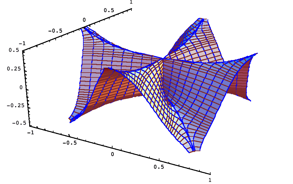
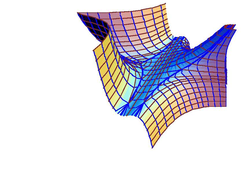
An Example From Differential Equations

Clay Ross (U. of the South, Sewanee, Tenn.) suggested the following: f(x, y) = x + x^2/2 - y + y^2/2 + log |x-1| + log |y+1|. The contour-flow image is more informative than a traditional plot. This surface arose from the separable differential equation, y' = x^2 (1 + y) / (y^2 (1-x)). Solutions to the diff. eqn. correspond to contours on the graph. From a geometrical perspective, the surface is interesting in that many of the flows dive into the origin, which is a saddle point.

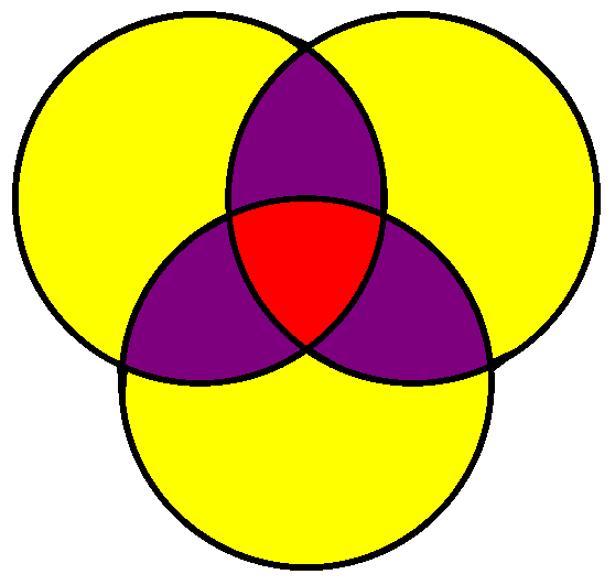
Rotationally Symmetric Venn Diagrams

Everyone knows the classic Venn diagram for 3 sets consisting of 3 circles.

This is rotationally symmetric and it is not hard to see that such can exist only when n is prime. The cases of 5 and 7 had been settled some time ago (when n = 5 one can do it with 5 ellipses), but the cases beyond that were challenging. Peter Hamburger obtained a rotationally symmetric Venn diagram when n = 11 in 2002, and more recently Griggs, Killian, and Savage showed that such exist for every prime. Much more information can be found in the excellent survey at <<http://www.combinatorics.org/Surveys/ds5/VennEJC.html>>

Using a Mathematica package I had written some years ago for four-coloring planar maps, I was able to manipulate the various maps and graphs used in these constructions, and so can present here the Venn diagram based on the Boolean structure of the dual found by Killian, Ruskey, Savage, and Weston, which is an extension of the GKS work.

Here is the map one first needs. This is a planar map with 2048 vertices (one is a point at infinity) and 1397 faces, and was found by KRSW. It is 4-colored using my 4-coloring algorithm. The dual of this map gives the Venn diagram.

Here is the dual to the Venn model, which is an exact Venn diagram. The map has 2048 regions, including the exterior, which corresponds to the empty set; there are 1397 intersections (out of a maximum possible 2046). They are colored according to Venn rank. This color scheme was worked out by Ruskey, Savage, and Wagon.

Here is one generator. Rotating this 10 times gives the 2048 regions.

And here is an image that combines everything. We see the Venn regions inside one generator only, and it is all superimposed on the 4-colored Venn model.

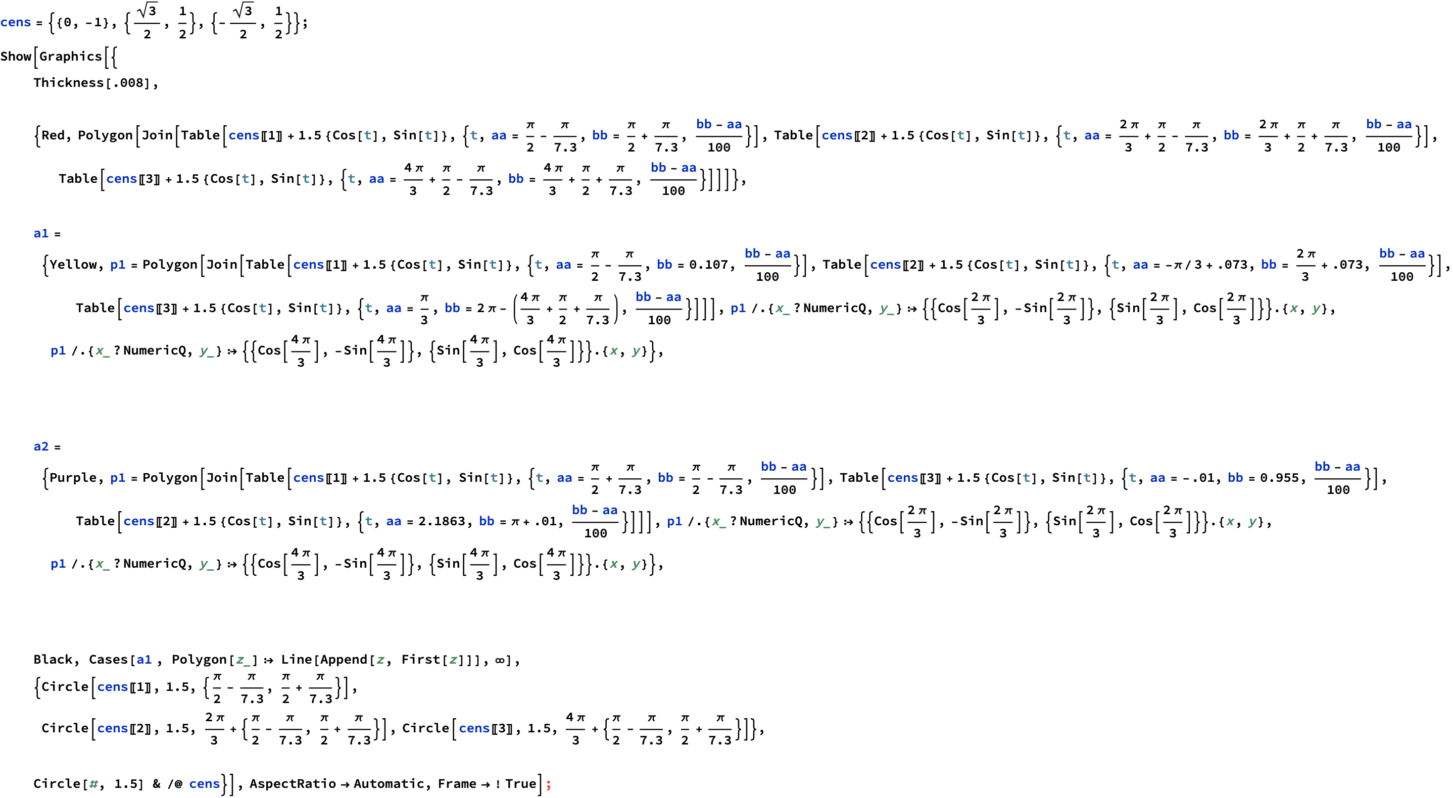
Code for Three

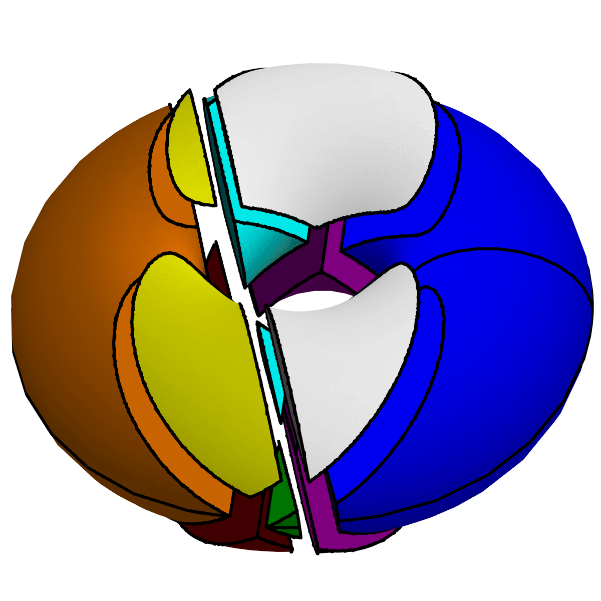
Cutting a Solid Torus into 13 Pieces