Solution
The problem was solved by Jia Tang, Richard Boardman, Michael Elgersma, Franz Pilcher, Michael Wyneken, Barry Cox, John Guilford, Bill Bass, Jack Ritter, and John Duncan.
This problem is quite well known, but yet the details were new to me, and to many of my readers. Thanks to Fuzzco's Josh Nissenboim for the suggestion.
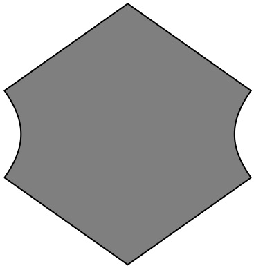
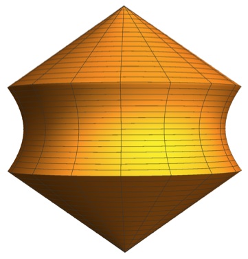
The solution is visible through these diagrams:


I found simple equations for the hyperbola at http://www.mathdemos.org/mathdemos/curvedcube/curvedcube.html
Bill Bass made a fantastic video by sticking an cube on the end of a drill. It is worth watching. Thanks, Bill.
The problem is a famous one. Matthew Wyneken (U Mich-Flint) observed:
For many years the late Dr. Paul Garlick of the University of Michigan-Flint posed this problem to his students. I learned it from him and realized that the answer was sitting on my desk — a hyperboloid made of string that I made as a boy after visiting the IBM Mathematics display at the Chicago Museum of Science and Industry sometime in late 1960's. So fascinated by the problem were his students that some of them made models to visualize what was happening.
So Bill Bass's model is one in a long line of such.
To see a movie in Mathematica, just evaluate the following code:
h[t_] := Which[0 <= t <= 1/Sqrt[3], t Sqrt[2], 1/Sqrt[3] < t < 2/Sqrt[3],
   Sqrt[2 t^2 - 2 t Sqrt[3] + 2], True, Sqrt[2] (Sqrt[3] - t)];

bd = Range[0,3] / Sqrt[3];

surf = Show[Table[RevolutionPlot3D[{h[t], t}, {t, bd[[i]], bd[[i+1]]},
ImageSize -> 600, Mesh -> {5, 20}, PlotPoints -> 50,
PlotStyle -> Opacity[0.46]], {i,3}], PlotRange -> All]

GT = GeometricTransformation; RT=RotationTransform;
Manipulate[Show[surf, Graphics3D[{
EdgeForm[{Thickness[0.02], Red}], FaceForm[Blue],
GT[GT[GT[Cuboid[], RT[ArcSec[Sqrt[3]], {1, 1, 0}]],
      TranslationTransform[{-0.78867, -0.2113, 0.57735}]],
      RT[\[Theta], {0, 0, 1}, {0, 0, 1}]]}],
Axes -> False, Boxed -> False, ViewPoint -> {0,-2.3,0},
PlotRange -> All], {\[Theta], 0., 2 Pi, 2 Pi/200}]
Version 10 of Mathematica has a new way of seeing these 3D objects that saves the user doing a lot of computation. One can define implicit regions, and take their union (or intersection, or difference), and then view them. This is extremely elegant, although images will be better when one has regions explicitly. Here are two examples: the union of the spun cubes, and also the intersection of the spun cubes (which is a bicone).
ang = ArcCos[1/Sqrt[3]];
rot[p_] := RotationMatrix[-ang, {1, 1, 0}] . p;
cen = {0.78867513459,0.21132486540,0}
spin[t_,p_] := (RotationMatrix[t, {0,0,1}] . (p-cen)) + cen
R1 = ImplicitRegion[ Thread[0 <= rot[{x,y,z}] <=1 ],  {x, y, z}];
reg[t_] := ImplicitRegion[ Thread[0 <= rot[ spin[t,{x,y,z}]]<=1], {x,y,z}];
reg[t] above gives the spun region through t radians. Now get the union and intersection:
un = RegionUnion @@ Table[reg[t] , {t, 0, 2 Pi / 3 , Pi / 50}];
in = RegionIntersection @@ Table[reg[t], {t, 0, 2 Pi / 3, Pi / 50}];
Now view them: The plotpoints setting gives better resolution, but is slow. Using 100 makes it slower still, and nicer. But the value in getting these regions in this implicit way is huge as a general technique.
RegionPlot3D[in, PlotPoints- > 50]
RegionPlot3D[un, PlotPoints -> 50]
[Back to Problem 1190]
© Copyright 2014 Stan Wagon. Reproduced with permission.